
improving contrast with the local laplacian filter
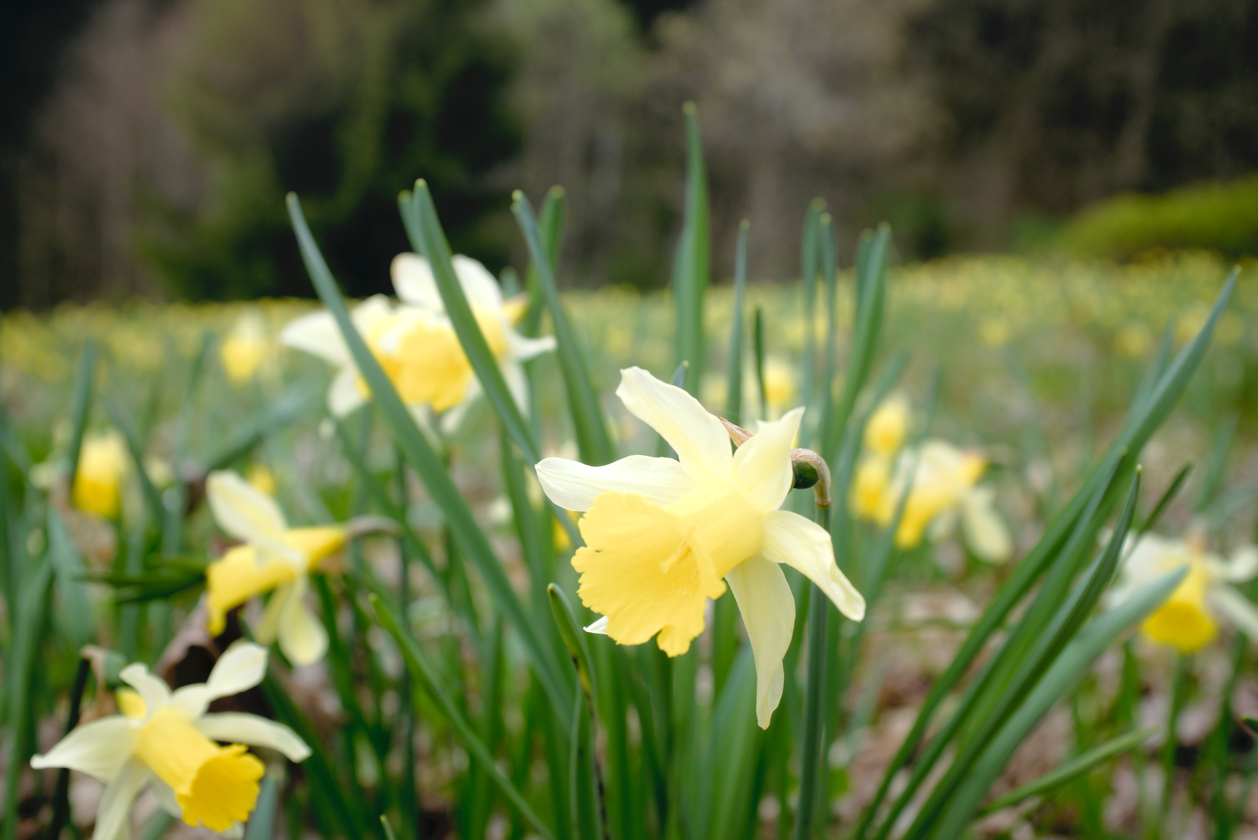
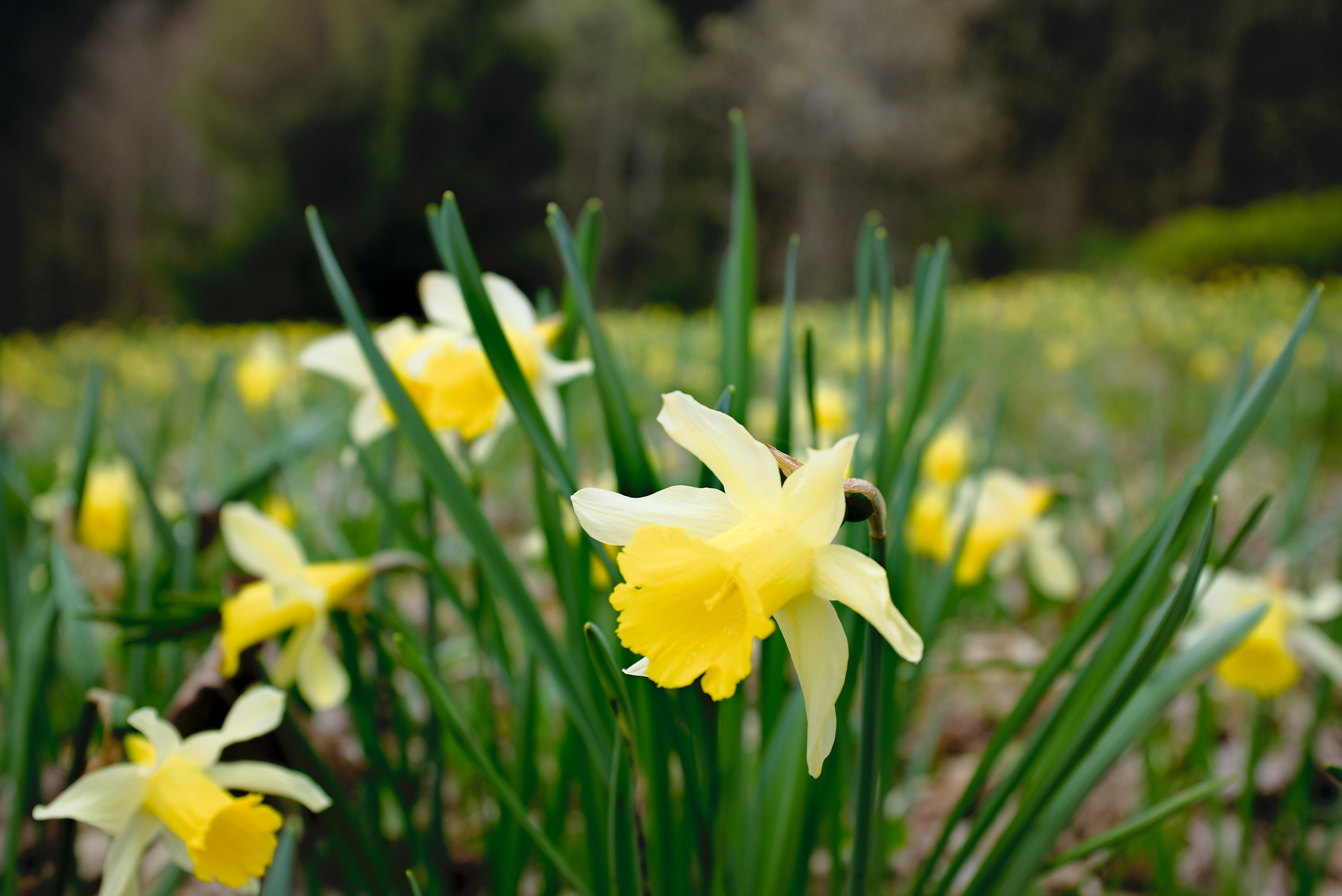
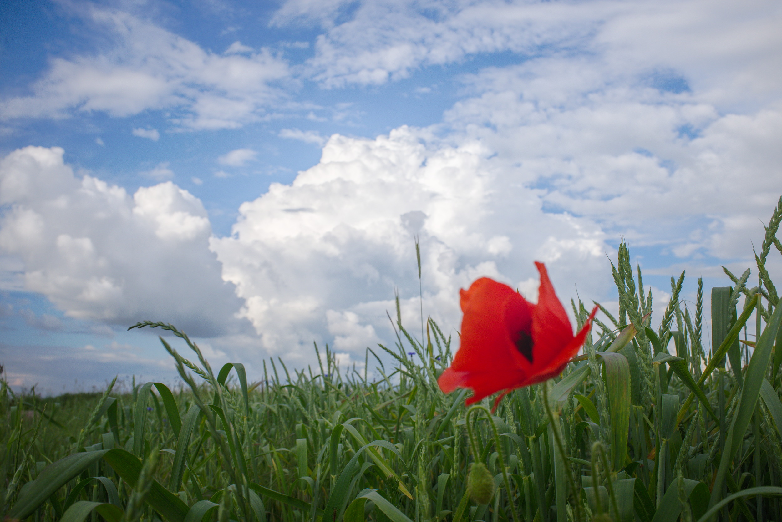
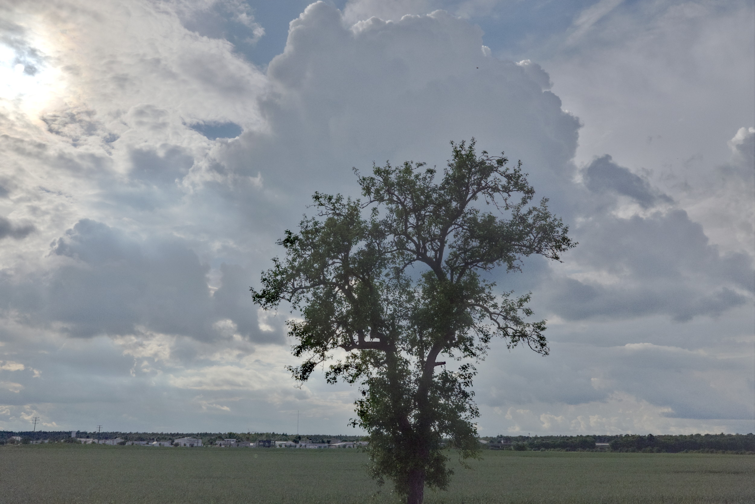
sometimes difficult lighting situations arise which, when taking photographs, result in unappealing pictures. for instance very uniform lighting on a cloudy day may give dull results, while very contrasty illumination (such as back lit) may require to compress the contrast to embrace both highlights and shadows in the limited dynamic range of the output device.
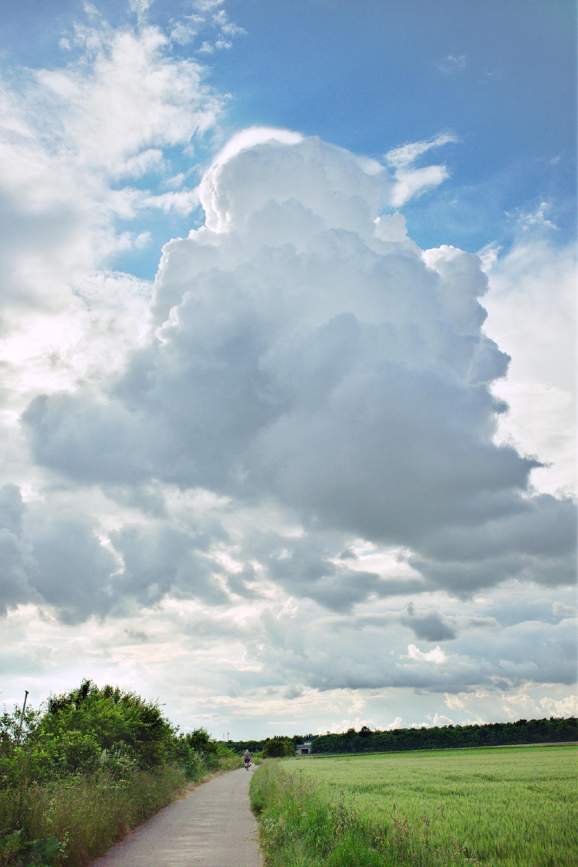
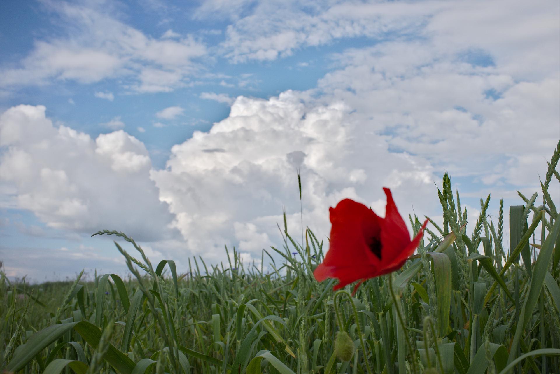
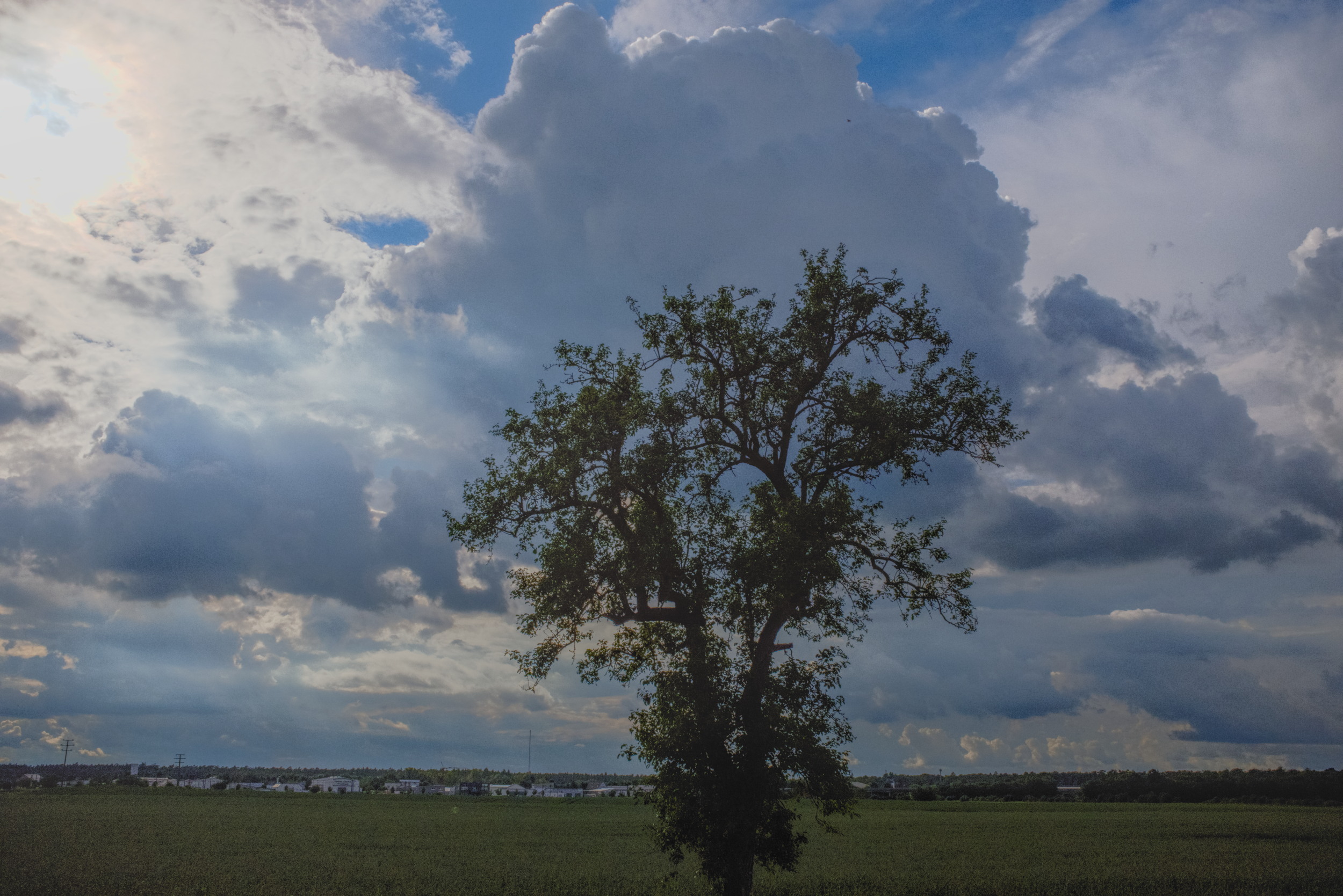
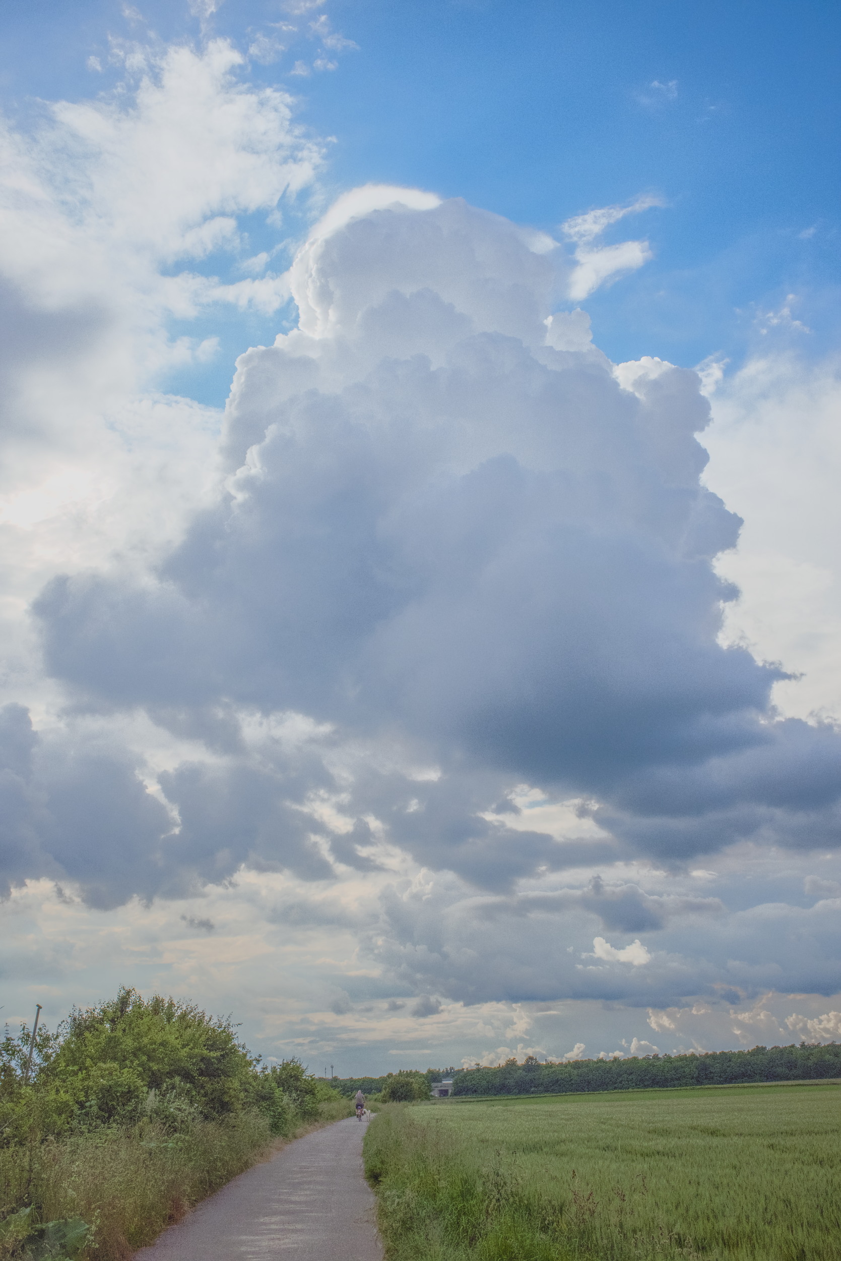
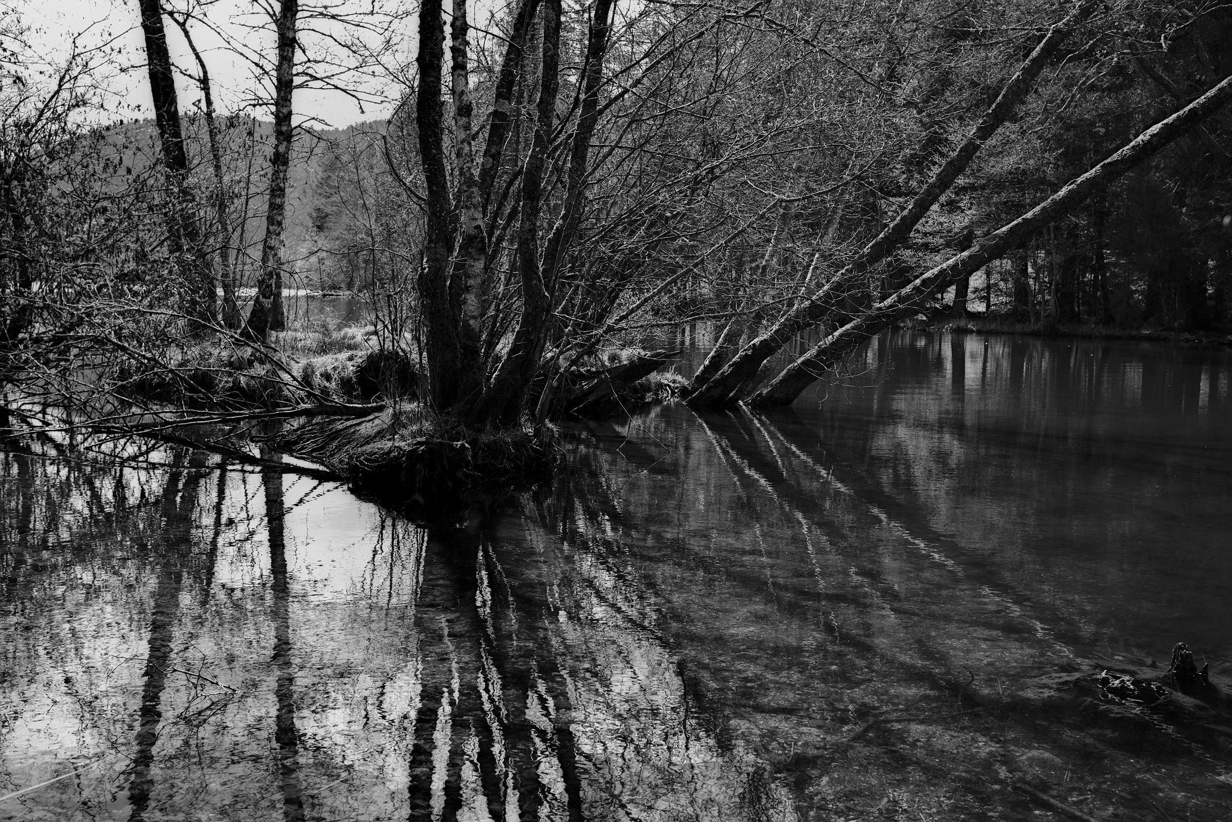
refer to the following two shots as examples:
- input + high contrast b/w
- hdr + compressed
many options to achieve this exist in literature and many of them are implemented in darktable already.
this post is about yet another approach to this which turned out to be extremely versatile, almost artifact-free, and reasonably fast to compute: the local laplacian pyramid.
repeat figure with curves and then it’s pretty much exposure fusion with many different images (one per gray level)
local contrast with the local laplacian pyramid
vanilla laplacian pyramids [0] are known to be a good tool to blend over between two images. for their applicability to local contrast, not so much. perhaps surprisingly, following up on exposure fusion (we blogged about that for darktable before ), a clever way to modify local contrast based on laplacian pyramids has been devised [1]: it works by pretty much creating a separate laplacian pyramid for every pixel in the image, and then selecting coefficients from these these based on certain criteria.
luckily, this can be reduced to processing the image only a small, fixed number of times [2]. the procedure is then basically:
- process the image n times, mapping it through a curve (see below for examples)
- create the n laplacian pyramids that go with the images
- merge into a final laplacian pyramid
- collapse this output pyramid to create the output image.
this is nicely illustrated in this video exported from halide:
also, as it turns out, the gpu is really good at processing laplacian pyramids. the opencl port of this turned out to be very useful.
the mapping function
why can we get away with this small fixed number n of processed pyramids? [2] gives the explanation in sec. 3:
If r is band-limited,
(r is the family of curves which is applied to the input image).
now if you look at the left image (which is taken from fig. 6 in [1]), it has clear kinks where the center part joints the straight lines. not band limited at all. don’t use this curve at home. it will produce random aliasing when used with the fast local laplacian code.
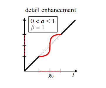

darktable uses what is shown on the right instead: the contrast-s curve in the center part is modelled by a derivative of gaussian (with infinite support), which is added to the straight lines on either side, which are blended over using a quadratic bezier curve. you can look up the precise code if you’re interested.
now changing the contrast-s curve in the middle changes local contrast, that’s great. looking at the sides of this curve, we would immediately want to use it for shadow lifting and highlight compression too. in fact that’s possible (see following section with images and accompanying curves). unfortunately some of the proposed optimisations in the original papers can’t be applied any more. for the shadow/highlight use case, the pyramid needs to be constructed all the way all the time, we can’t stop after three levels (or else the shadow lifting would depend on the scale of the image).
this means darktable will always build the full pyramids, making this a little slower, but yielding best results.
the darktable ui
you can find our implementation of this filter in the local contrast module, when
switched to local laplacian mode:
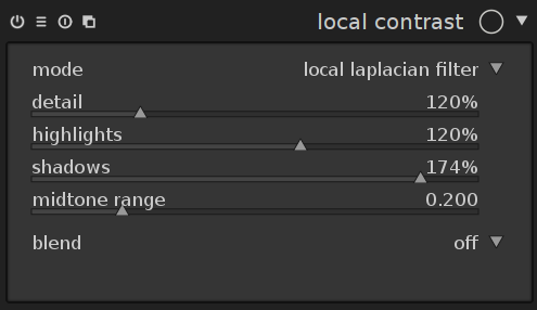
it allows you to change detail (or clarity or local contrast), highlight contrast, and shadow contrast separately. the last slider governs how wide the central region of the curve is, i.e. what is classified as shadow vs. mid-tone.
in the following, we’ll go through these contrast sliders, showing a couple of corresponding conversion curves and the resulting effect on the output image.
drag the separator in the middle to compare before/after!
increased local contrast:

pulled highlights down:
yes, the curve changes the bottom part. which you would think belongs to the shadows. turns out it doesn’t.

pushed shadows up:

inverse of the above
and the inverse is also possible, top to bottom, left to right: original, removed details, pushed highlights out even more, pulled shadows deeper.
application to hdr compression
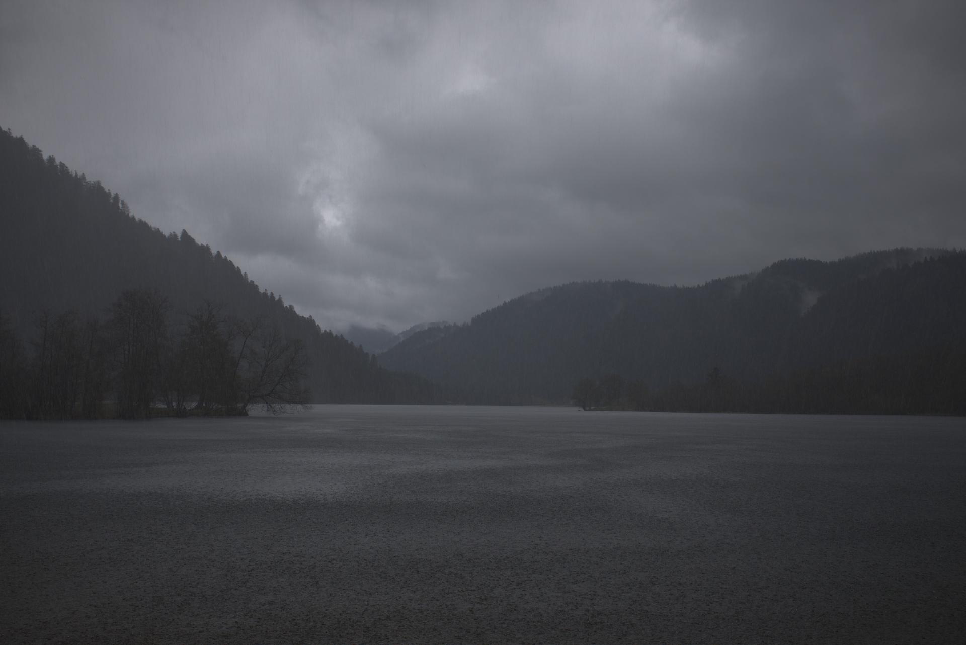
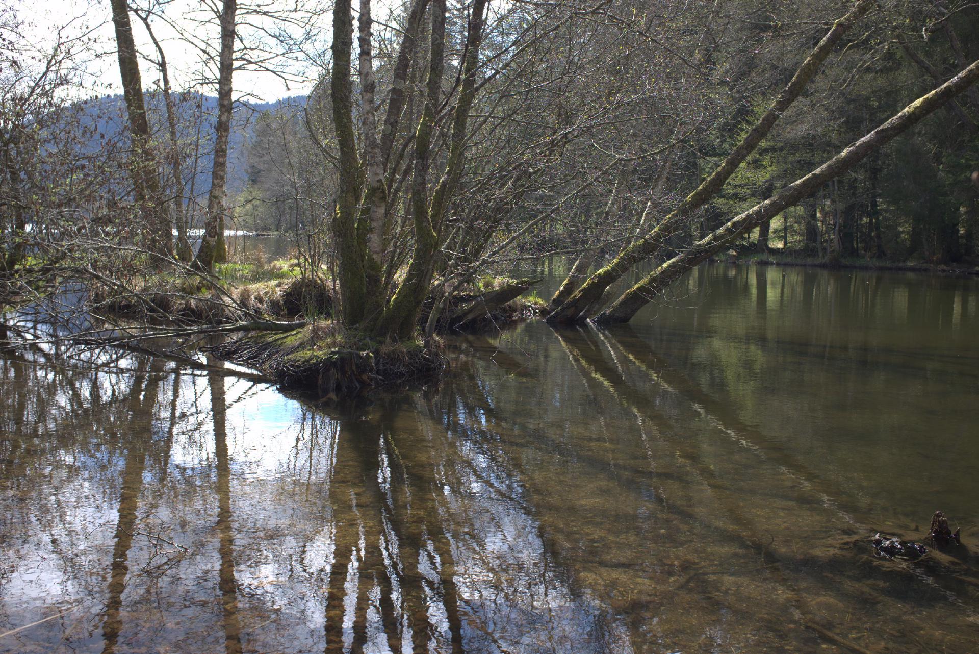
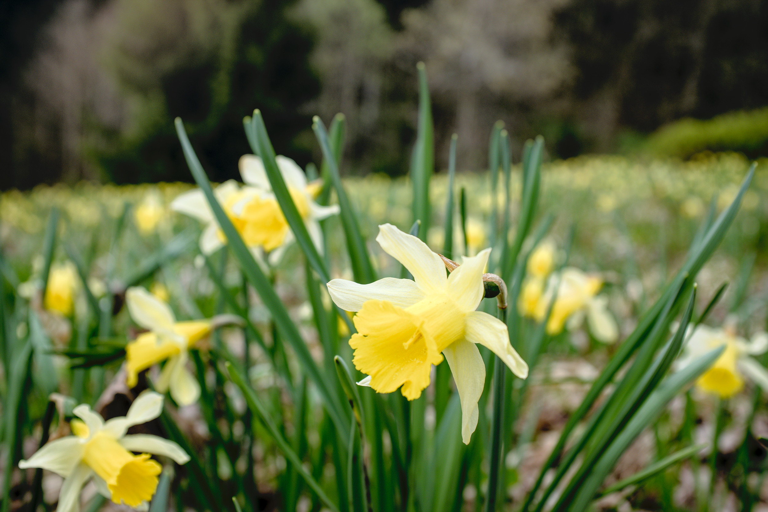
in the following there are some comparison images from the previous post on exposure fusion. these have been processed again with a different approach:
- to compress the dynamic range, a very flat base curve has been used which maxes out at 0.5 for input values of 1.0.
- as contrast-s curve, the tone curve module has been used, in rgb mode for automatic colour saturation compensation.
- the curve was created to match an out of camera raw+jpg pair using
darktable-chartwhich also created a clut for the colour lookup table module.
this approach will leave the image flat and dull (due to the flat base curve). to add back additional detail, we use the local laplacian module. this turns out to work a lot better together with a contrast-s tone curve than with a contrast-s base curve, since the base curve comes before the local contrast module in the pipeline, while the tone curve comes after. this way, the local contrast module receives more linear input.
in fact, sometimes a contrast-s curve is not necessary at all for hdr input. exposure fusion shows some nicer behaviour with respect to colour saturation at times, but sometimes produces halo like artifacts. i find it easier to create good results with the local laplacian when aiming for a low key look (see the definition in the darker clouds in the left of the first image). really up to you and any given input images which method works better.
example history stacks are in the example comparison images seen below: 0 1 2.

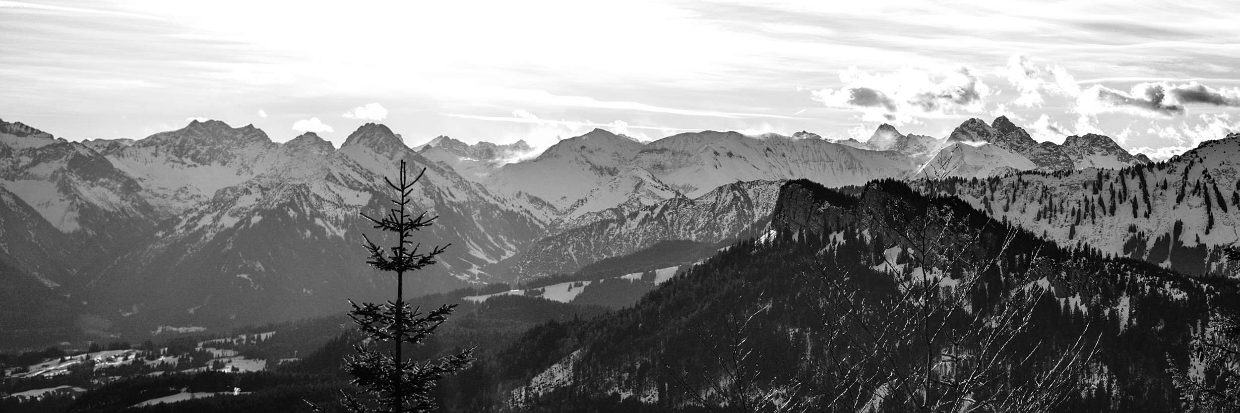
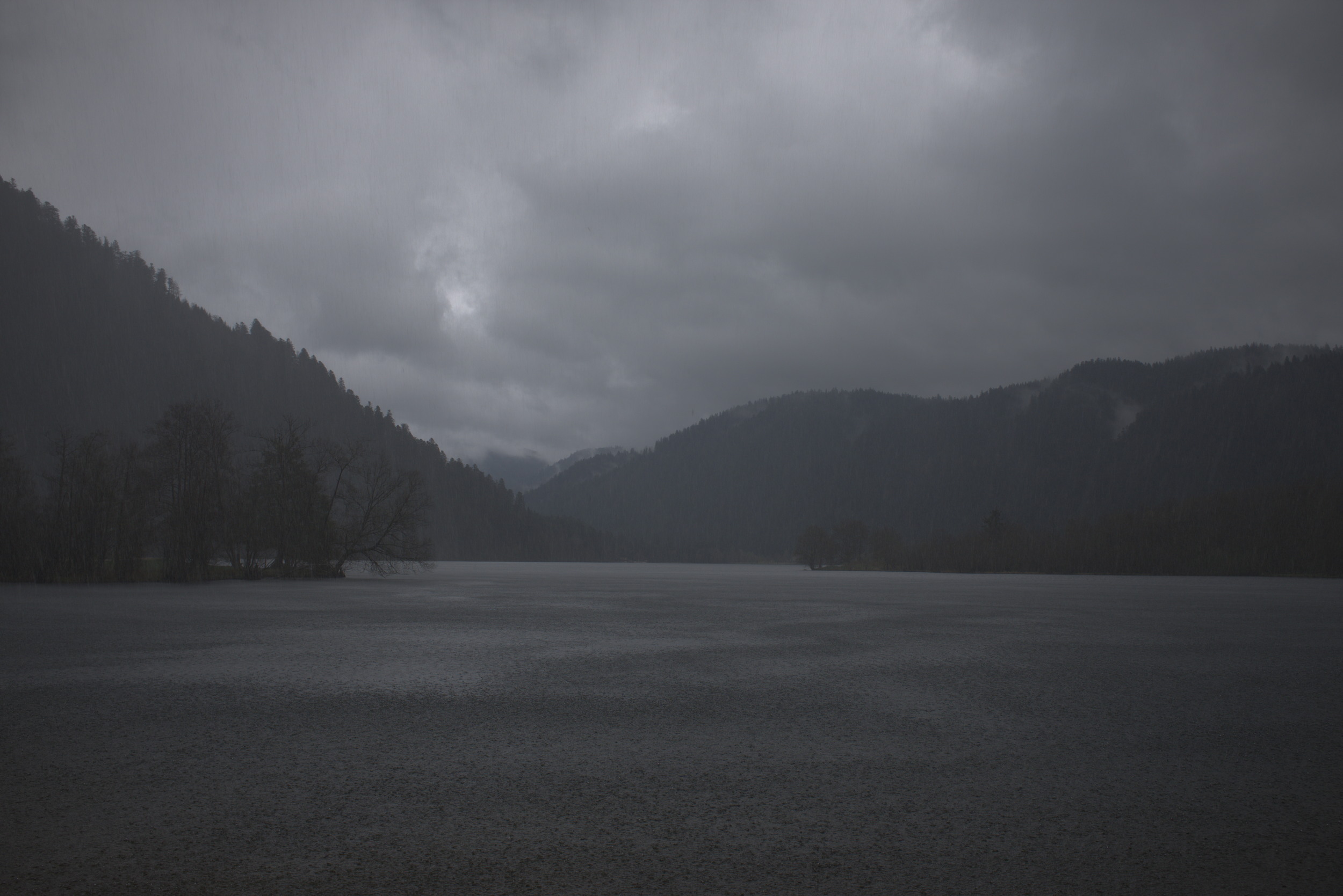
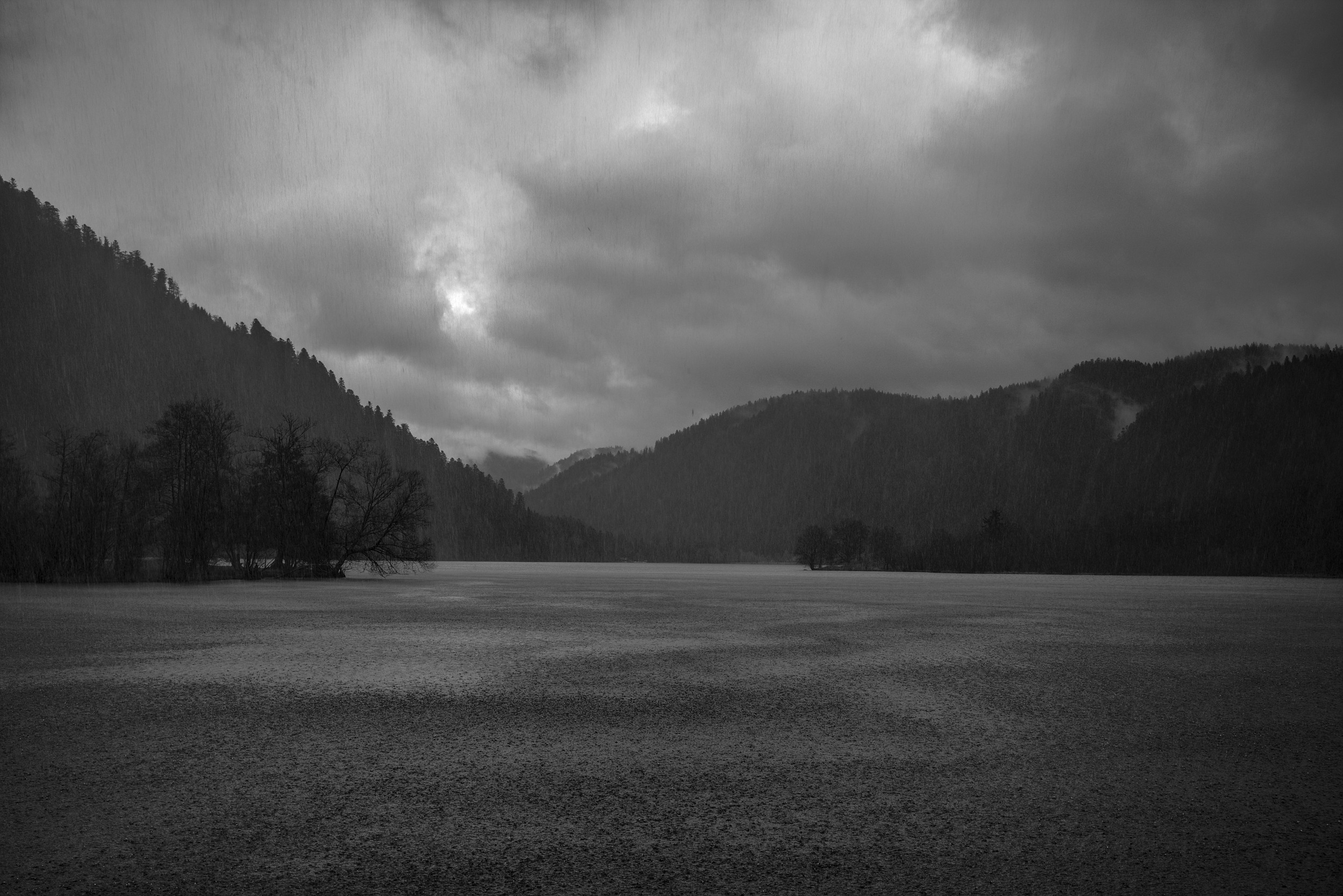
application to high contrast monochrome
a note on noise
when increasing contrast, you want to make sure the input isn’t noisy, or else that noise would be accentuated even more. but even when not increasing contrast, the local laplacian filter will show structured artifacts for noisy input. i find this mostly goes away when enabling at least chroma denoising for instance in the profiled denoising module.

