in an ideal world, an image is piecewise smooth. it has soft gradients, some detail and edges. in particular there’s no noise and the edges are sharp. given these assumptions, you can do a lot of cool things to your pictures, using techniques like frequency space editing, wavelets, or local histograms.

darktable’s equalizer module demonstrates some of this, using the wavelet approach. you can use it to sharpen and denoise, enhance or attenuate certain frequencies in your image, while keeping the edges intact.

today’s blog post is about a different technique which does similar things, and i’ll demonstrate a few usecases in our new pipeline.

bilateral filter

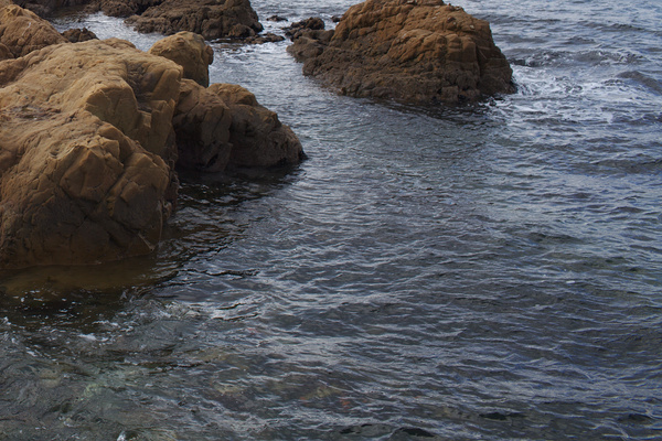
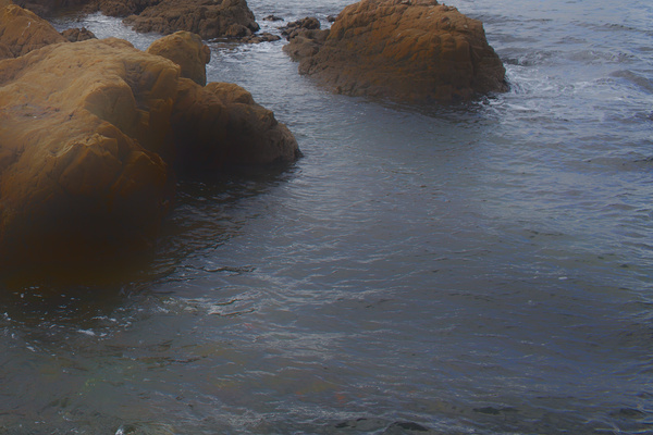
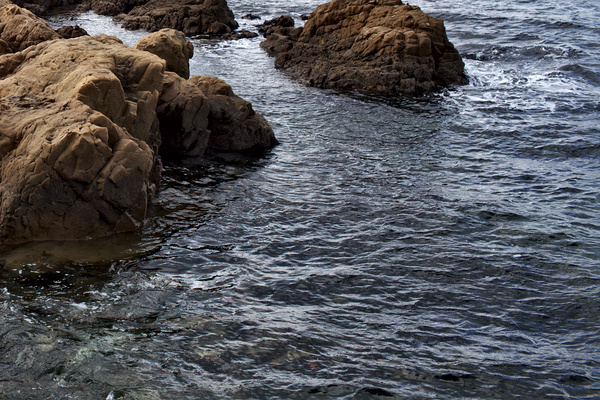
a bilateral filter is basically a high dimensional gaussian blur, which can be evaluated very quickly at reasonable memory cost (and with a simple implementation) if you limit yourself to 3d (pixel position and brightness) [0]. this is what it looks like (left: original, right: bilateral filter applied):

a bit boring, eh? while we actually use this filter for denoising in one of our modules (in 5d and using the permutohedral lattice [1] instead of the grid), it’s mainly useful as a building block (base layer for local contrast enhancement etc).

importance of edges

take local contrast enhancement as an example. it works much like the standard `unsharp mask sharpening’ filter. first you blur your picture to get a smooth base layer, subtract it from the original, and add back the difference (containing all the small detail) multiplied with a contrast boost value > 1.

let’s do this on a one dimensional line. the following graphs show a 1d signal I (red), the blurred base layer B (green), the detail D (difference between the two, blue), and the signal after local contrast enhancement B + 2 D (magenta):

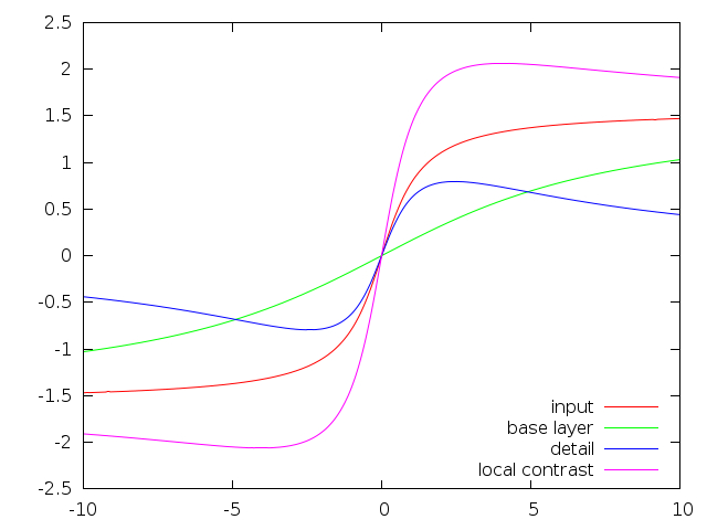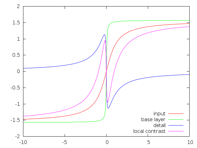the left graph shows an overblurred base layer, the right one is too sharp (the edge is almost a step function, no smooth gradient). for local contrast enhancement we’d actually like to keep the edges as they are, so these curves should all line up perfectly (and detail should be zero), we only want to enhance small structures, not change edges.

so what happens is the left picture will produce large halos (bright sky will get too bright close to the edge, and then too dark on the other side before averaging out), while the right one shows ugly gradient reversals, which will show up as a double line close to edges.

this problem has been described and solved automatically by [2], and our equalizer module has the `sharpness’ curve for you to take care of this manually. but there’s also a possibility to make the bilateral filter a little more well-behaved with respect to this, while actually making the implementation faster [3]. there are other/newer techniques to fix this, but these are somewhat more heavy weight (local laplacians).

implementation

our implementation of the 3d unnormalized bilateral grid is straight forward, not particularly optimized and very fast. especially for large sigma the number of grid points is very low and thus the blur step doesn’t have a lot of work to do.

the only difference to a regular bilateral grid is the third blur step, which blurs along the dimension of brightness. instead of blurring it with a gaussian, a kernel that looks very similar to the derivative of a gaussian is used. this leads to what is better described in [3], that the effect of the filter is toned down at the edges instead of being normalized to a weight of 1.0, leading in a slightly uninformed result. more precisely, take the bilateral filter $B_p$ at pixel p:

$$B_p = \frac{1}{W_p} \sum_q I_q G_{\sigma_r}(|| I_q - I_p ||) G_{\sigma_s}(||q-p||)$$

$$\mbox{ with } W_p = \sum_q G_{\sigma_r}(|| I_q - I_p ||) G_{\sigma_s}(||q-p||),$$

and the unnormalized variant:

$$B’p = I_p + \sum_q (I_q-I_p) G{\sigma_r}(|| I_q - I_p ||) G_{\sigma_s}(||q-p||).$$

pulling $I_p$ out of the sum is just a no-op. the interesting part is leaving away the division by the weight. for small values of the two gaussians, this results in a very low magnitude of the sum overall, effectively leaving the input image $I_p$ unchanged. this happens near edges, where only half the neighbourhood is considered close by with respect to the range sigma. the awesome side effect is that we don’t have to compute $W_p$.

during the first phase, splatting, we need to rasterize the 3d points in the input image into the downsampled grid. this turns out to be a synchronization problem when using a lot of threads (on the gpu). this still results in underwhelming performance after some shared memory tricks. our opencl implementation thus detects the gpu at compile time and uses inline ptx assembly for nvidia’s floating point atomics in global memory. as a reference for all the poor guys who need the same instruction in opencl and don’t feel like digging through the manuals, here it is:

asm volatile ("atom.global.add.f32 %0, [%1], %2;" : "=f"(res) : "l"(val), "f"(delta));

with that, my GT 540M achieves an acceptable 2-3x speedup over my core i7 @2GHz (note: totally unoptimized non-SIMD implementation), depending on input parameters (sigma totally change the way sync problems arise).

examples

now for some pictures. i said it’s going to be useful as a building block, here are some use cases.

monochrome

in this Lab colorspace module, L is multiplied with a color filter value based on the ab channels. the problem here is noisy input and unstable color channels around very dark or very bright areas, or even worse at the transition between those. effectively, the noisy L channel is multiplied by correlated noise in the ab channels, which literally multiplies noise (left image below). the new code computes color filter values, smoothes them (in an edge aware way) and then applies the rest of the filter as before (right image).

tone mapping

the module `global tonemapping’ has lost the meaning of its title, and got an additional slider to add more local detail. please don’t push it all the way to the right (or else we delete your image).

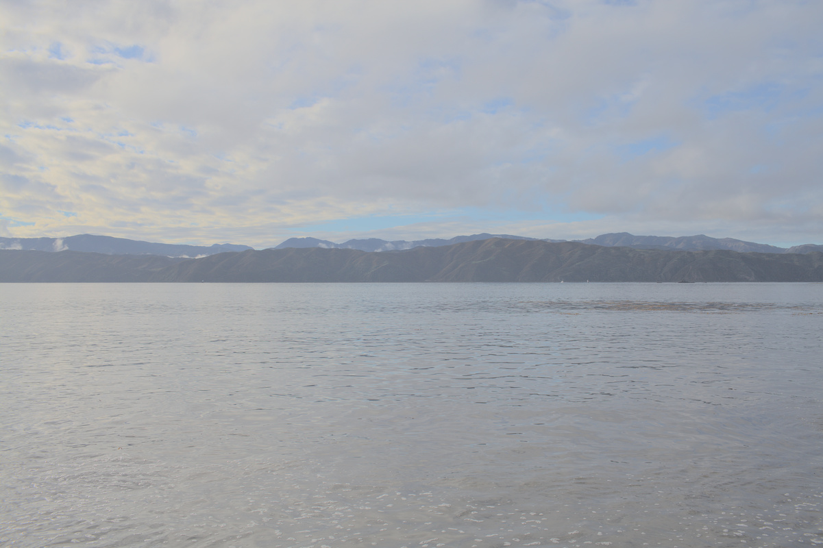
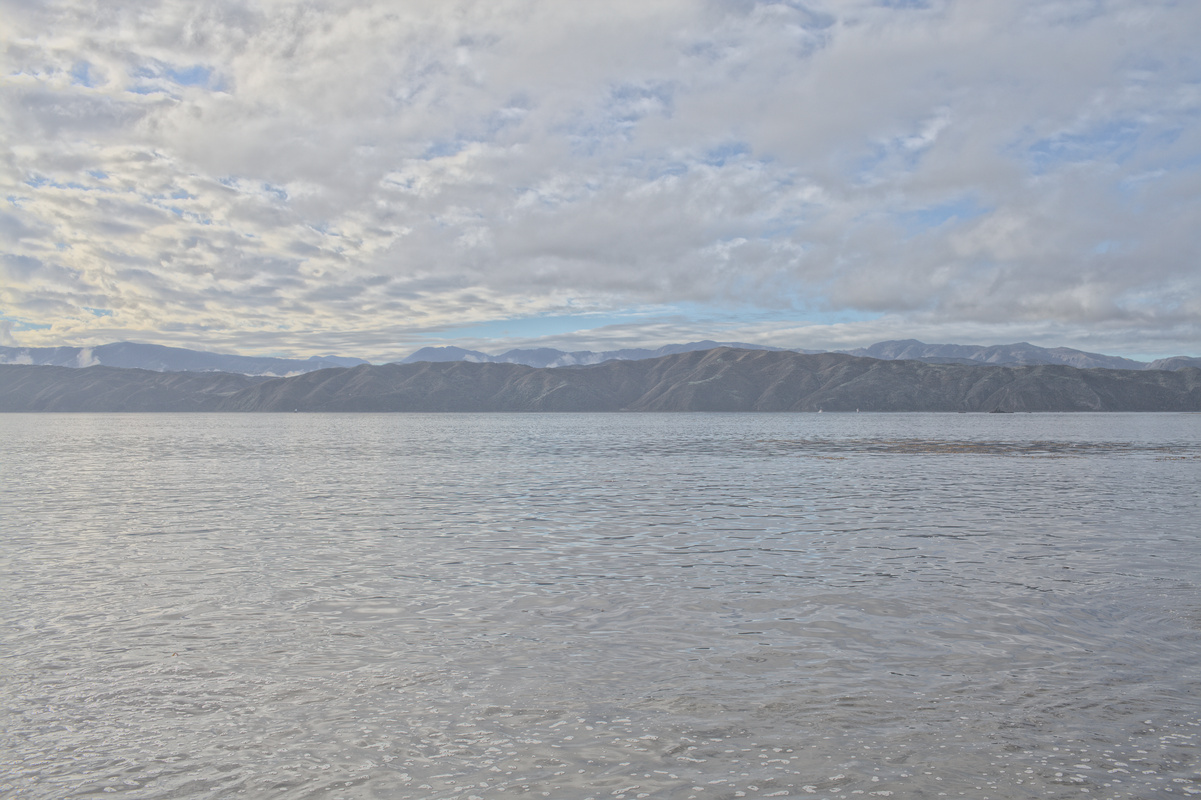
this example has been treated with the `filmic response curve’ and lost a lot of contrast in the process. the right version has some of it added back, and will result in this common cheap hdr look that you’ll find everywhere around the web if you push it any more (just ours comes without the halos i guess).

shadows/highlights

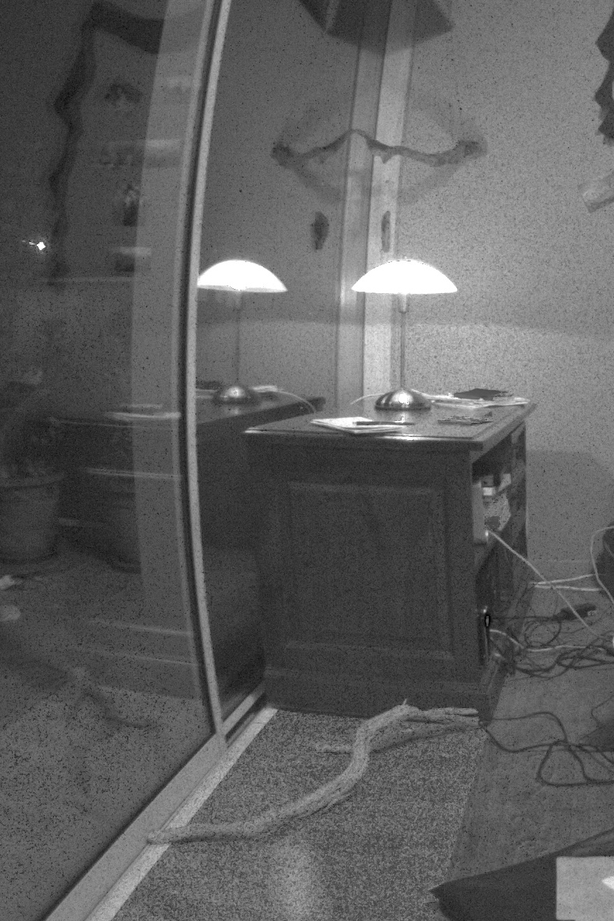
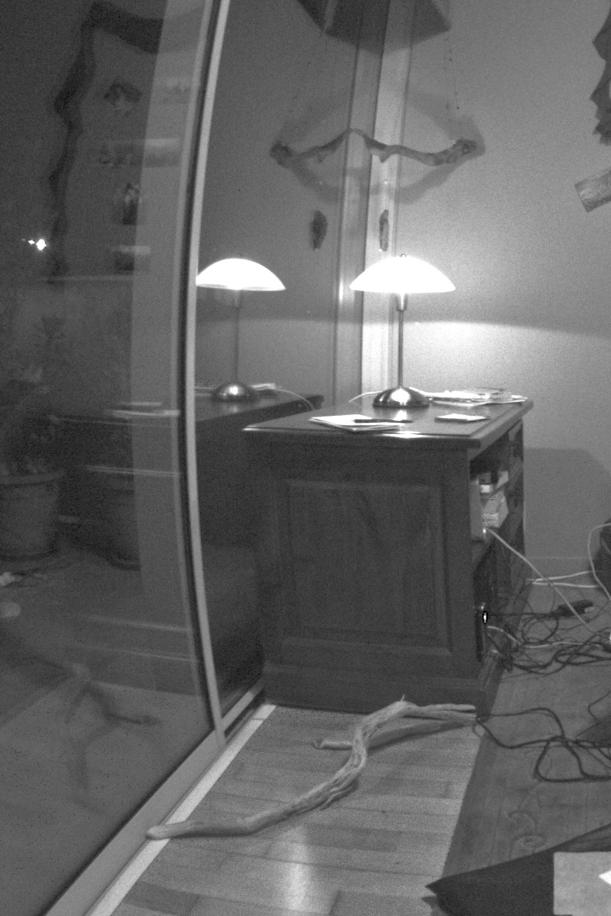
this module makes use of a lowpass filter to achieve a consistent shadow recovery operation. on high contrast edges, it can suffer from halos, so it now has the option to switch from pure lowpass (gaussian) to edge aware (bilateral filter). the difference is illustrated in the following three pictures (original, gaussian, bilateral):

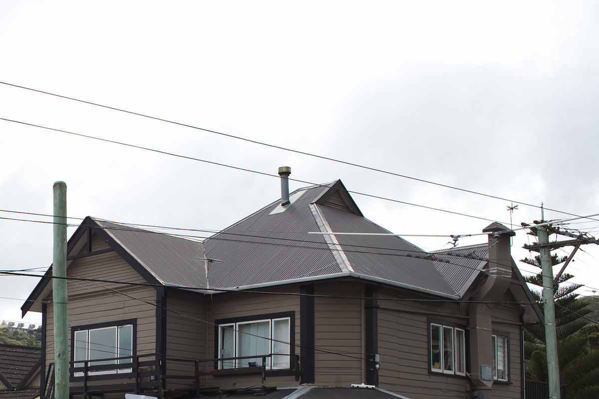
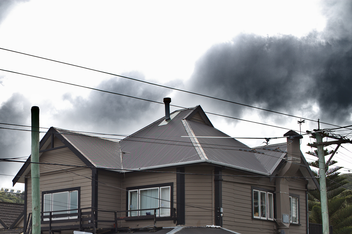
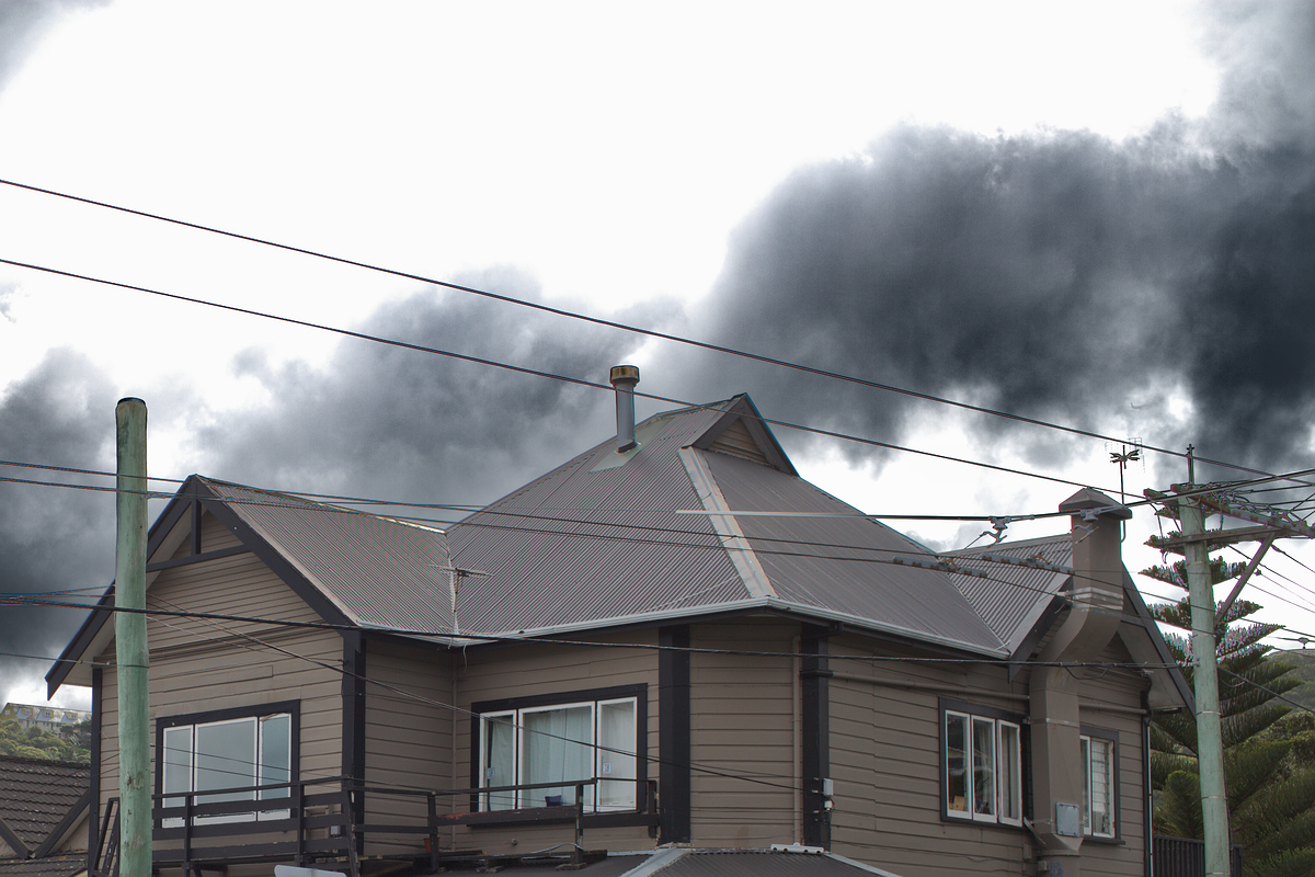
this image had the highlights toned down quite a bit to exaggerate the effect. note the strong halos around the roof and the darkening of the top of this pole at the left.

we left you with a choice between the two mainly for backwards compatibility (quite a big difference). but it is also worth noting that sometimes the bilateral filtering fails in the sense that it doesn’t correctly detect coloured edges (chromatic aberrations anyone?) or sometimes still results in oversharpening as described above. all of that is mainly visible if you push your highlights/shadows so hard that the image will be destroyed for that reason already (like my example above), but you never know. if working with the bilateral option, be sure to double check your edges.

more

this might be useful to increase the stability of blend-if masks in the future. i’m not aware of any problems there, but if they arise we know what to do.

there is the possibility of a standalone bilateral local contrast tool with a reasonably low amount of edge artifacts. it currently sits in the `bilateral’ branch because we already have so many modules and i’m not sure how useful it is. as a teaser, you can do the following to a 1Mpix image in 20ms on an i7:

references

• [0] Real-Time Edge-Aware Image Processing with the Bilateral Grid. Jiawen Chen, Sylvain Paris, Frédo Durand, 2007.
• [1] Fast High-Dimensional Filtering Using the Permutohedral Lattice. Andrew Adams, Jongmin Baek, Abe Davis. 2010.
• [2] Smoothed Local Histogram Filters. Michael Kass, Justin Solomon. 2010.
• [3] Fast and Robust Pyramid-based Image Processing. Mathieu Aubry, Sylvain Paris, Samuel Hasinoff, Jan Jautz, Frédo Durand. 2011.